practice - torch sklearn numpy

practice - torch sklearn numpy#

sklearn, numpy for linear regression and gradient descent

kaggle House Prices - Advanced Regression Techniques에서 가져온 데이터를 이용하여, Linear Regression을 구현해보자.

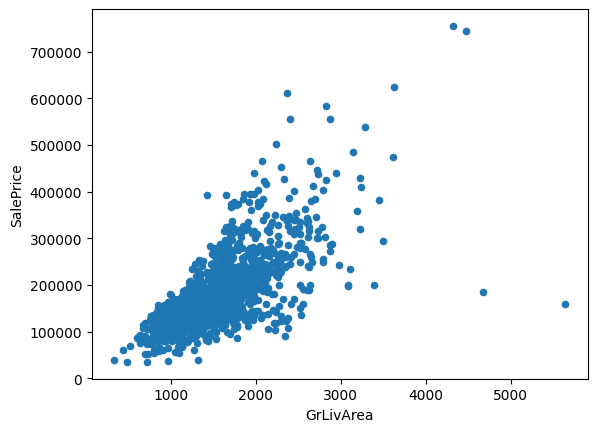
우리의 SalesPrice가 구하기를 원하는 y이고 이것은 연속적인(continuous)한 value이기 때문에 linear regression을 사용하는 과제라고 볼 수 있다. GriLivArea(Above grade(ground) living area square feet)은 cs229에서 말하는 size(feet^2)와 가장 유사한 column이라고 생각되어서 뽑았다. 단순하게 scatter plot을 해봐도 사이드로 많이 빠진 몇 outlier들을 제외하면 어느 정도의 linear 관계를 볼 수 있을 거라고 생각된다.

import pandas as pd
import numpy as np
import matplotlib.pyplot as plt
from sklearn.linear_model import LinearRegression
from IPython.display import display, Markdown

train = pd.read_csv('./files/train.csv')
train

	Id	MSSubClass	MSZoning	LotFrontage	LotArea	Street	Alley	LotShape	LandContour	Utilities	...	PoolArea	PoolQC	Fence	MiscFeature	MiscVal	MoSold	YrSold	SaleType	SaleCondition	SalePrice
0	1	60	RL	65.0	8450	Pave	NaN	Reg	Lvl	AllPub	...	0	NaN	NaN	NaN	0	2	2008	WD	Normal	208500
1	2	20	RL	80.0	9600	Pave	NaN	Reg	Lvl	AllPub	...	0	NaN	NaN	NaN	0	5	2007	WD	Normal	181500
2	3	60	RL	68.0	11250	Pave	NaN	IR1	Lvl	AllPub	...	0	NaN	NaN	NaN	0	9	2008	WD	Normal	223500
3	4	70	RL	60.0	9550	Pave	NaN	IR1	Lvl	AllPub	...	0	NaN	NaN	NaN	0	2	2006	WD	Abnorml	140000
4	5	60	RL	84.0	14260	Pave	NaN	IR1	Lvl	AllPub	...	0	NaN	NaN	NaN	0	12	2008	WD	Normal	250000
...	...	...	...	...	...	...	...	...	...	...	...	...	...	...	...	...	...	...	...	...	...
1455	1456	60	RL	62.0	7917	Pave	NaN	Reg	Lvl	AllPub	...	0	NaN	NaN	NaN	0	8	2007	WD	Normal	175000
1456	1457	20	RL	85.0	13175	Pave	NaN	Reg	Lvl	AllPub	...	0	NaN	MnPrv	NaN	0	2	2010	WD	Normal	210000
1457	1458	70	RL	66.0	9042	Pave	NaN	Reg	Lvl	AllPub	...	0	NaN	GdPrv	Shed	2500	5	2010	WD	Normal	266500
1458	1459	20	RL	68.0	9717	Pave	NaN	Reg	Lvl	AllPub	...	0	NaN	NaN	NaN	0	4	2010	WD	Normal	142125
1459	1460	20	RL	75.0	9937	Pave	NaN	Reg	Lvl	AllPub	...	0	NaN	NaN	NaN	0	6	2008	WD	Normal	147500

1460 rows × 81 columns

train[['SalePrice','GrLivArea']].plot.scatter(x='GrLivArea', y='SalePrice')

<Axes: xlabel='GrLivArea', ylabel='SalePrice'>

../../_images/184e93a7308b6cd2c24649a1102013af9c8f3cb9c1d326ab306cf92ac26926b4.png

standardization#

\[\begin{equation*} z = \frac{x - \mu}{\sigma} \end{equation*}\]

$\mu$는 평균, $\sigma$는 표준편차
$z$는 표준화된 값으로, 평균으로부터 얼마나 떨어져 있으며, 그 거리를 표준편차의 몇 배수만큼 떨어져 있는지를 나타낸다.
데이터를 평균이 0이고, 표준편차가 1인 값으로 변환하는 것.
데이터의 범위를 일정하게 조정하고, 다양한 스케일을 가진 변수들간 비교 가능하도록 만듦.
outlier에 영향을 받을 수 있기 때문에 데이터의 분포에 따라 (가우시안 normal distribution이 아닐 경우) 다른 scaler를 사용해야 할 수 있다.
입력변수 X를 standardization 하지 않고 학습할 경우에 가중치의 값이 제대로 학습되지 않을 수 있다. 스케일이 다르기 때문에.

X = train['GrLivArea'].values.reshape(-1,1)
y = train['SalePrice'].values.reshape(-1,1)
X = (X - X.mean()) / X.std()
y = (y - y.mean()) / y.std()

Sklearn linear regression#

lr = LinearRegression()
lr.fit(X, y)
y_pred = lr.predict(X)

plt.scatter(X, y)
plt.plot(X, y_pred, color='red')
plt.show()

# print("$h(\Theta)$" f"= {lr.coef_[0][0]:.2f}x + {lr.intercept_[0]:.2f}")
result_str =  r"$h(\Theta)$ = {:.2f}x + {:.2f}".format(lr.coef_[0][0], lr.intercept_[0])
display(Markdown(result_str))

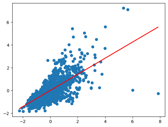
../../_images/3a267dd826cff982539876f3baddaeea105fcc73f945d4fb5ed675c8c8d0e9b0.png

$h(\Theta)$ = 0.71x + 0.00

Numpy implementation#

lr = 1e-1
n_epochs = 5000
a = np.random.randn(1)
b = np.random.randn(1)

for epoch in range(n_epochs):
    y_hat = a + b * X
    error = y - y_hat
    loss = (error**2).mean()

    a_grad = -2 *error.mean()
    b_grad = -2 * (X * error).mean()

    a = a - lr * a_grad
    b = b - lr * b_grad
    
result_str =  r"$h(\Theta)$ = {:.2f}x + {:.2f}".format(b[0], a[0])
display(Markdown(result_str))